Chapter 48 Topic Modelling

Topic modeling is a method for unsupervised classification of documents, similar to clustering on numeric data, which finds natural groups of items even when we’re not sure what we’re looking for.

Latent Dirichlet allocation (LDA) is a particularly popular method for fitting a topic model. It treats each document as a mixture of topics, and each topic as a mixture of words. This allows documents to “overlap” each other in terms of content, rather than being separated into discrete groups, in a way that mirrors typical use of natural language.

################################################################################################

#Topic Modelling with Simpsons

#########################################################################################
SC = ScriptsCharacters %>%
   select(id,name,normalized_text)

corpus = Corpus(VectorSource(SC$normalized_text))

# Pre-process data
corpus <- tm_map(corpus, tolower)

corpus <- tm_map(corpus, removePunctuation)

corpus <- tm_map(corpus, removeWords, stopwords("english"))

corpus <- tm_map(corpus, removeWords, UniqueLowIDF[1:500])

corpus <- tm_map(corpus, stemDocument)

dtm = DocumentTermMatrix(corpus)

# Remove sparse terms
dtm = removeSparseTerms(dtm, 0.997)

# Create data frame
labeledTerms = as.data.frame(as.matrix(dtm))

labeledTerms = labeledTerms[rowSums(abs(labeledTerms)) != 0,]

##############################################################################
#LDA Modelling Starts
###############################################################################

# set a seed so that the output of the model is predictable
simpsons_lda <- LDA(labeledTerms, k = 2, control = list(seed = 13))

#The tidytext package provides this method for extracting the per-topic-per-word probabilities, 
# called   β  (“beta”), from the model
simpsons_topics <- tidy(simpsons_lda, matrix = "beta")

simpsons_top_terms <- simpsons_topics %>%
  group_by(topic) %>%
  top_n(10, beta) %>%
  ungroup() %>%
  arrange(topic, -beta)

simpsons_top_terms %>%
  mutate(term = reorder(term, beta)) %>%
  ggplot(aes(term, beta, fill = factor(topic))) +
  geom_col(show.legend = FALSE) +
  facet_wrap(~ topic, scales = "free") +
  coord_flip() + theme_bw()

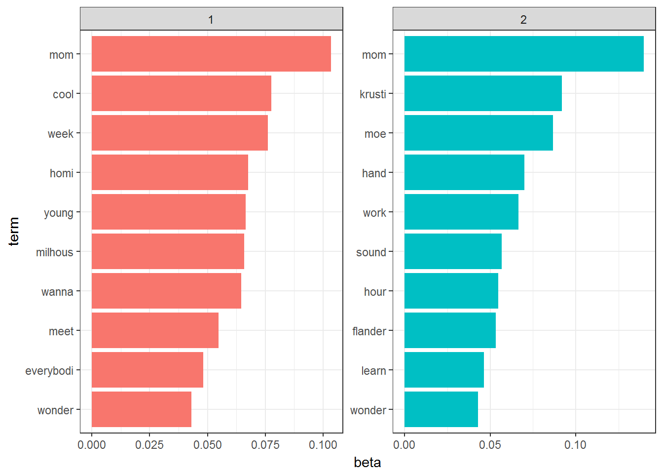
This visualization lets us understand the two topics that were extracted from the Script Lines.

The most common words in topic 1 include mom,homi,milhous which suggests it may represent the Simpson family topics.

Those most common in topic 2 include moe,work,hour suggesting that this topic represents work related things.

One important observation about the words in each topic is that some words, such as wonder, are common within both topics. This is an advantage of topic modeling as opposed to “hard clustering” methods: topics used in natural language could have some overlap in terms of words.