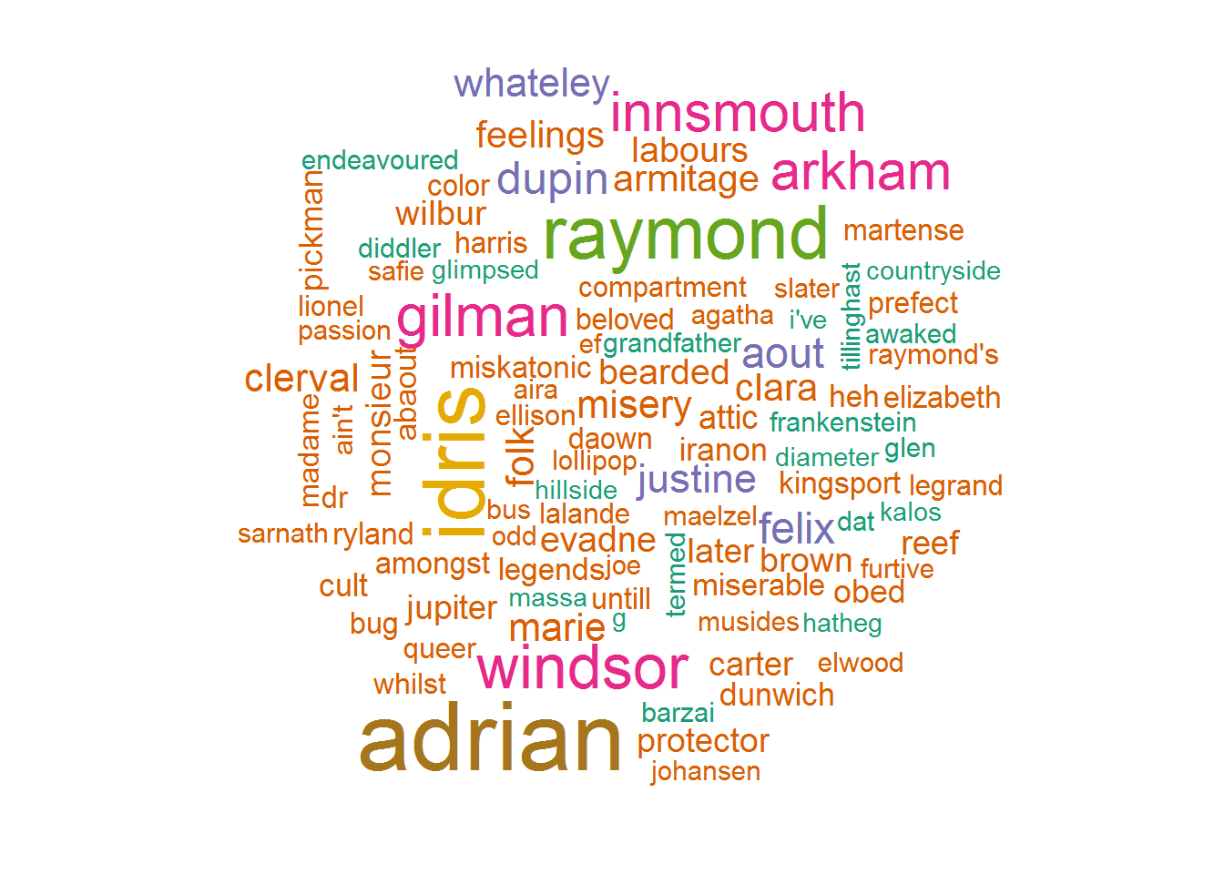
Chapter 9 TF-IDF

We wish to find out the important words which are written by the authors. Example for your young child , the most important word is mom. Example for a bar tender , important words would be related to drinks.

We would explore this using a fascinating concept known as Term Frequency - Inverse Document Frequency. Quite a mouthful, but we will unpack it and clarify each and every term.

A document in this case is the set of lines written by an author.

Therefore we have different documents for each Author.

From the book 5 Algorithms Every Web Developer Can Use and Understand

TF-IDF computes a weight which represents the importance of a term inside a document.

It does this by comparing the frequency of usage inside an individual document as opposed to the entire data set (a collection of documents). The importance increases proportionally to the number of times a word appears in the individual document itself–this is called Term Frequency. However, if multiple documents contain the same word many times then you run into a problem. That’s why TF-IDF also offsets this value by the frequency of the term in the entire document set, a value called Inverse Document Frequency.

9.1 The Math

TF(t) = (Number of times term t appears in a document) / (Total number of terms in the document)
IDF(t) = log_e(Total number of documents / Number of documents with term t in it).
Value = TF * IDF

9.2 Twenty Most Important words

Here using TF-IDF , we investigate the Twenty Most Important words

trainWords <- train %>%
  unnest_tokens(word, text) %>%
  count(author, word, sort = TRUE) %>%
  ungroup()

total_words <- trainWords %>% 
  group_by(author) %>% 
  summarize(total = sum(n))

trainWords <- left_join(trainWords, total_words)

#Now we are ready to use the bind_tf_idf which computes the tf-idf for each term. 
trainWords <- trainWords %>%
  filter(!is.na(author)) %>%
  bind_tf_idf(word, author, n)

   
plot_trainWords <- trainWords %>%
  arrange(desc(tf_idf)) %>%
  mutate(word = factor(word, levels = rev(unique(word))))

plot_trainWords %>% 
  top_n(20) %>%
  ggplot(aes(word, tf_idf)) +
  geom_col(fill = fillColor) +
  labs(x = NULL, y = "tf-idf") +
  coord_flip() +
  theme_bw()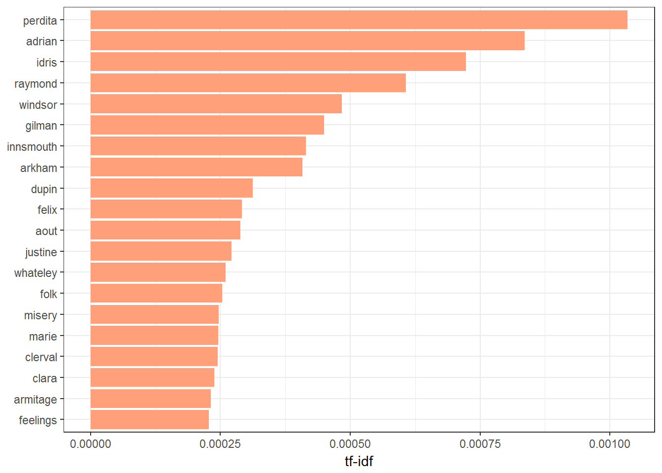

9.2.1 Twenty most important words HPL

plot_trainWords %>%
  filter(author == 'HPL') %>%
  top_n(20) %>%
  ggplot(aes(word, tf_idf)) +
  geom_col(fill = fillColor2) +
  labs(x = NULL, y = "tf-idf") +
  coord_flip() +
  theme_bw()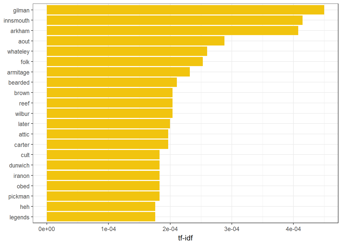

9.2.2 Twenty most important words EAP

plot_trainWords %>%
  filter(author == 'EAP') %>%
  top_n(20) %>%
  ggplot(aes(word, tf_idf)) +
  geom_col(fill = fillColor) +
  labs(x = NULL, y = "tf-idf") +
  coord_flip() +
  theme_bw()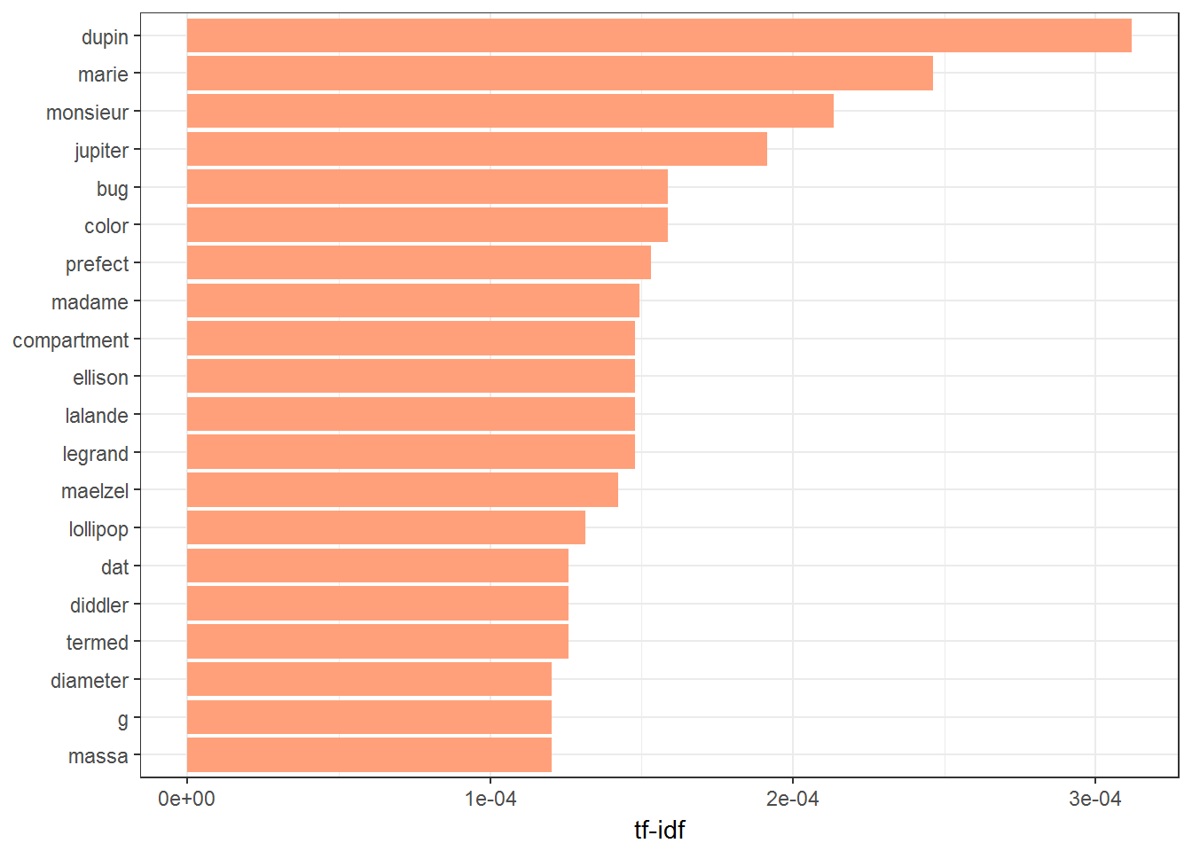

9.2.3 Twenty most important words MWS

plot_trainWords %>%
  filter(author == 'MWS') %>%
  top_n(20) %>%
  ggplot(aes(word, tf_idf, fill = author)) +
  geom_col() +
  labs(x = NULL, y = "tf-idf") +
  coord_flip() +
  theme_bw()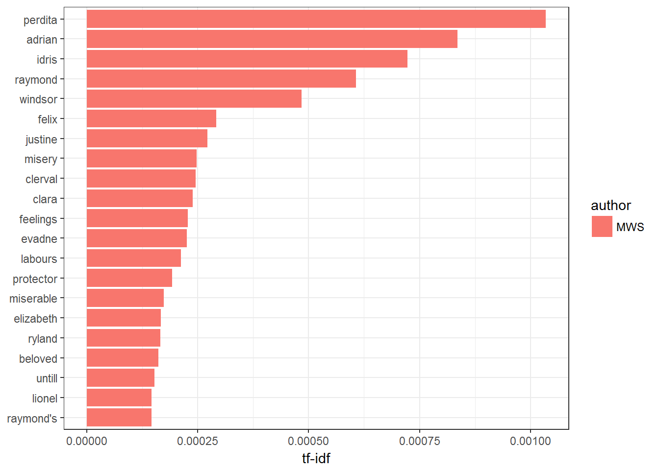

9.3 Word Cloud for the Most Important Words

We show the Hundred most important words. This Word Cloud is based on the TF- IDF scores. Higher the score, bigger is the size of the text.

plot_trainWords %>%
  with(wordcloud(word, tf_idf, max.words = 100,colors=brewer.pal(8, "Dark2")))