Chapter 44 Top Twenty most Common Words

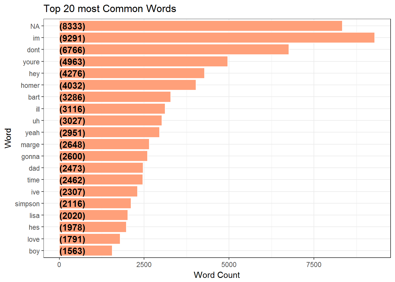
We examine the Top Twenty Most Common words and show them in a bar graph.

SC = ScriptsCharacters %>%
   select(id,name,normalized_text)

SC %>%
  unnest_tokens(word, normalized_text) %>%
  filter(!word %in% stop_words$word) %>%
  dplyr::count(word,sort = TRUE) %>%
  ungroup() %>%
  mutate(word = factor(word, levels = rev(unique(word)))) %>%
  head(20) %>%
  
  ggplot(aes(x = word,y = n)) +
  geom_bar(stat='identity',colour="white", fill =fillColor) +
  geom_text(aes(x = word, y = 1, label = paste0("(",n,")",sep="")),
            hjust=0, vjust=.5, size = 4, colour = 'black',
            fontface = 'bold') +
  labs(x = 'Word', y = 'Word Count', 
       title = 'Top 20 most Common Words') +
  coord_flip() + 
  theme_bw()

44.1 WordCloud of the Common Words

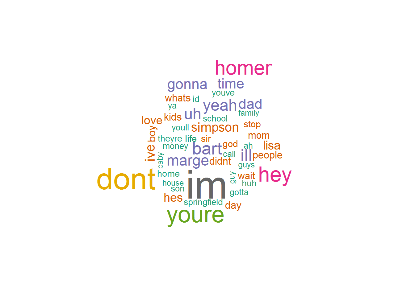
A word cloud is a graphical representation of frequently used words in the Normalized text. The height of each word in this picture is an indication of frequency of occurrence of the word in the entire text.
im , dont , hey and homer are some of the most commonly occuring terms.

SC %>%
  unnest_tokens(word, normalized_text) %>%
  filter(!word %in% stop_words$word) %>%
  dplyr::count(word,sort = TRUE) %>%
  ungroup()  %>%
  head(50) %>%
  
  with(wordcloud(word, n, max.words = 50,colors=brewer.pal(8, "Dark2")))