Chapter 31 Distribution of Mass

Here Mass is a continous variable and therfore for the distribution we plot a histogram.

We plot the distribution of the Mass of the Meteorites.

MetLandings %>%
    ggplot(aes(x = mass) )+
    geom_histogram(fill = fillColor2) +
    scale_x_log10() +
    scale_y_log10() + 
    labs(x = 'Mass in gms' ,y = 'Count', title = paste("Distribution of", "mass")) +
    theme_bw()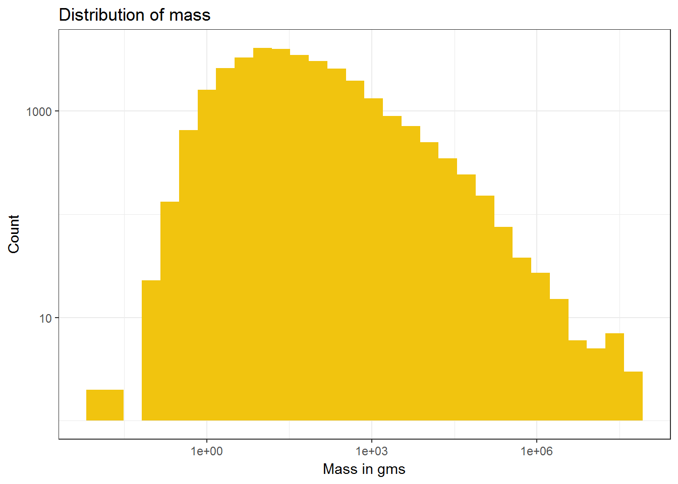

31.1 Heaviest Meteorite

The mass is in Kilograms.

MetHeaviest =  max(MetLandings$mass,na.rm = TRUE)

MetHeviestRec = MetLandings %>%
  filter(mass == MetHeaviest) %>%
  mutate( mass = mass/1e3)

kable(MetHeviestRec,"html") %>%
  kable_styling(bootstrap_options = c("striped", "hover", "condensed", "responsive")) %>%
  scroll_box(width = "800px")

name	id	nametype	recclass	mass	fall	year	reclat	reclong	GeoLocation
Hoba	11890	Valid	Iron, IVB	60000	Found	1920	-19.58333	17.91667	(-19.583330, 17.916670)

31.2 Lightest Meteorite

The mass is in Kilograms.

MetLightest =  min(MetLandings$mass,na.rm = TRUE)

MetLightestRec = MetLandings %>%
  filter(mass == MetLightest) %>%
  mutate( mass = mass/1e3)

kable(head(MetLightestRec,6),"html") %>%
  kable_styling(bootstrap_options = c("striped", "hover", "condensed", "responsive")) %>%
  scroll_box(width = "800px")

name	id	nametype	recclass	mass	fall	year	reclat	reclong	GeoLocation
Gove	52859	Relict	Relict iron	0	Found	1979	-12.26333	136.83833	(-12.263330, 136.838330)
Österplana 048	56147	Relict	Relict OC	0	Found	2004	58.58333	13.43333	(58.583330, 13.433330)
Österplana 049	56148	Relict	Relict OC	0	Found	2012	58.58333	13.43333	(58.583330, 13.433330)
Österplana 050	56149	Relict	Relict OC	0	Found	2003	58.58333	13.43333	(58.583330, 13.433330)
Österplana 051	56150	Relict	Relict OC	0	Found	2006	58.58333	13.43333	(58.583330, 13.433330)
Österplana 052	56151	Relict	Relict OC	0	Found	2006	58.58333	13.43333	(58.583330, 13.433330)

31.3 Valid Lightest Meteorite

The mass is in Kilograms.

MetLandingsValid = MetLandings %>%
  filter(nametype == 'Valid')

MetLightest =  min(MetLandingsValid$mass,na.rm = TRUE)

MetLightestRec = MetLandingsValid %>%
  filter(mass == MetLightest) %>%
  mutate( mass = mass/1e3)


kable(head(MetLightestRec,6),"html") %>%
  kable_styling(bootstrap_options = c("striped", "hover", "condensed", "responsive")) %>%
  scroll_box(width = "800px")

name	id	nametype	recclass	mass	fall	year	reclat	reclong	GeoLocation
Yamato 8333	29438	Valid	H5	1e-05	Found	1983	-71.5	35.66667	(-71.500000, 35.666670)

31.4 Distribution of Mass classified by Fall Type

31.4.1 Autoselect Fall Type Colors

We plot the distribution of the Mass of the Meteorites based on their Fall Type

MetLandings %>%
      ggplot(aes(x = mass, fill = fall)) +
      geom_histogram(alpha = 0.8) +
      scale_x_log10() +
      scale_y_log10() + 
      labs(x= 'Mass in gms',y = 'Count', title = paste("Distribution of", ' mass ')) +
      theme_bw()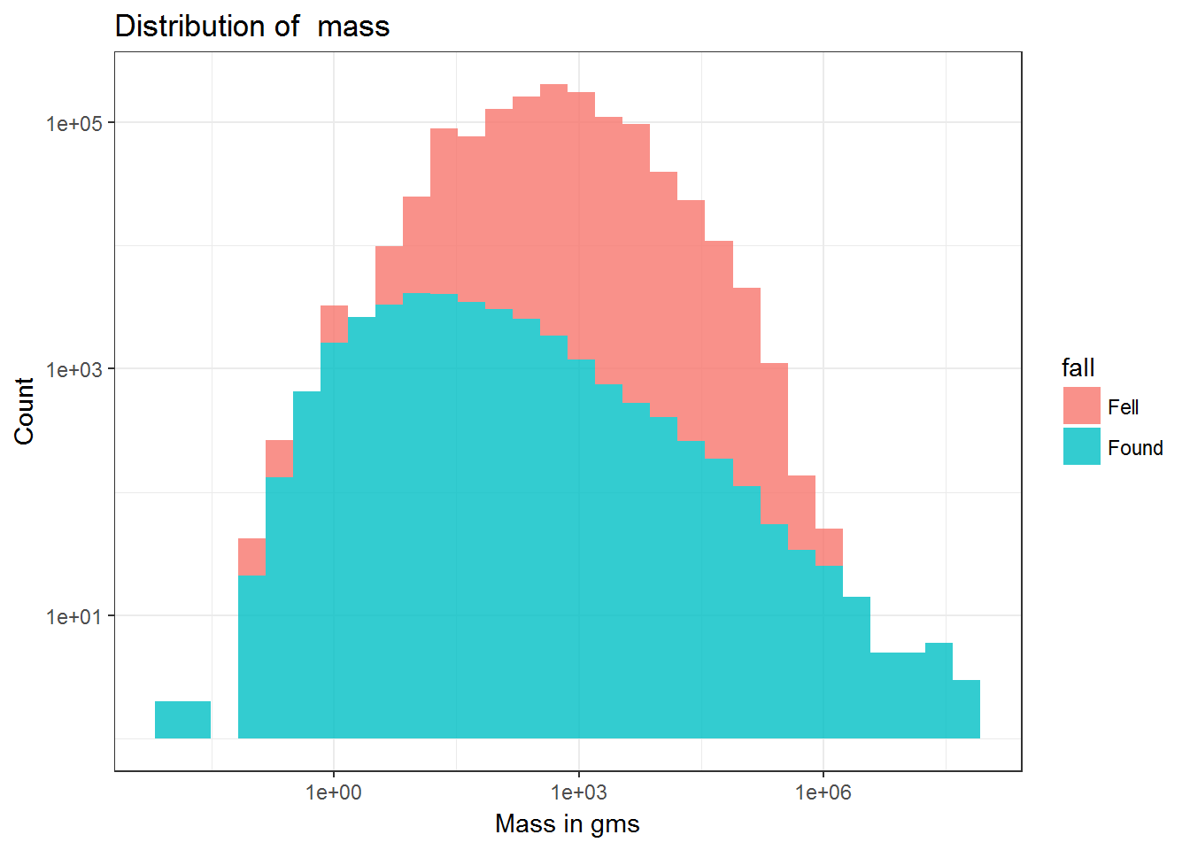

31.4.2 Select Fall Type Colors

We plot the distribution of the Mass of the Meteorites based on their Fall Type. Here we manually select the colors of the fall type.

MetLandings %>%
  
    ggplot(aes(x = mass, fill = fall)) +    
  
      geom_histogram(alpha = 0.8) +
      scale_x_log10() +
      scale_y_log10() + 
      
      scale_fill_manual( values = c("red","blue") )+
  
      labs(x= 'Mass in gms',y = 'Count', title = paste("Distribution of", ' mass ')) +
      theme_bw()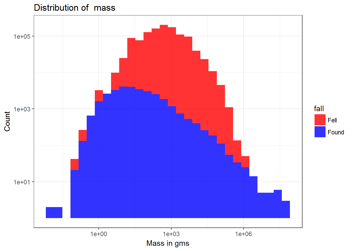

31.5 Mass with plots for each fall Type

Here Mass is a continous variable and Fall is a categorical variable. To examine the relationships between a continous and categorical variable, we plot a facet bar plot.

MetLandings %>%
  
      ggplot(aes(x = mass, fill = fall)) +    
      geom_histogram(alpha = 0.8) +
      scale_x_log10() +
      scale_y_log10() + 
      
      scale_fill_manual( values = c("red","blue") ) +
      facet_wrap(~fall) +
  
      labs(x= 'Mass in gms',y = 'Count', title = paste("Distribution of", ' mass ')) +
      theme_bw()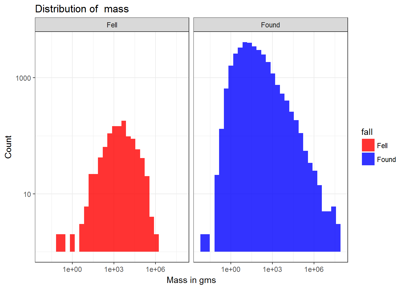

31.6 Mass with plots for each fall Type

Here Mass is a continous variable and Fall is a categorical variable. To examine the relationships between a continous and categorical variable, we plot a BoxPlot plot.

In this case, we do a BoxPlot with the mass being transformed into Kilograms. The plot shows a number of outliers and the distribution of the mass for each fall type is not very clearly observed.

MetLandings %>%
  mutate( fill = as.factor(fall)) %>%
      ggplot(aes(x = fall, y= mass/1e3, fill = fall)) +
      geom_boxplot() +
      scale_fill_manual( values = c("red","blue") ) +
  
      facet_wrap(~fall) +
  
      labs(x= 'Fall Type',y = 'Mass in Kgs', title = paste("Distribution of", ' mass ')) +
      theme_bw()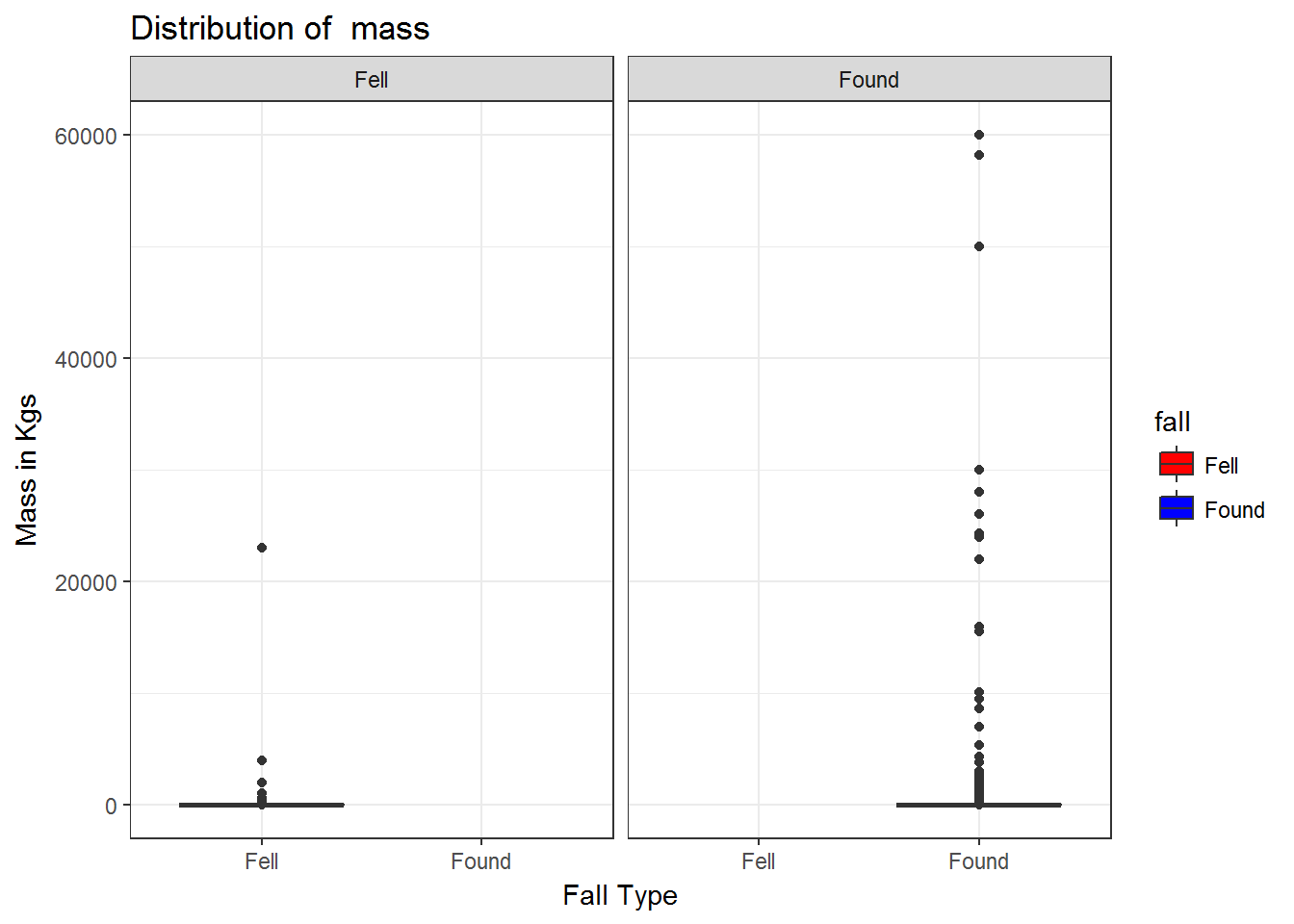

31.7 Mass with plots for each fall Type ( partially removing outliers)

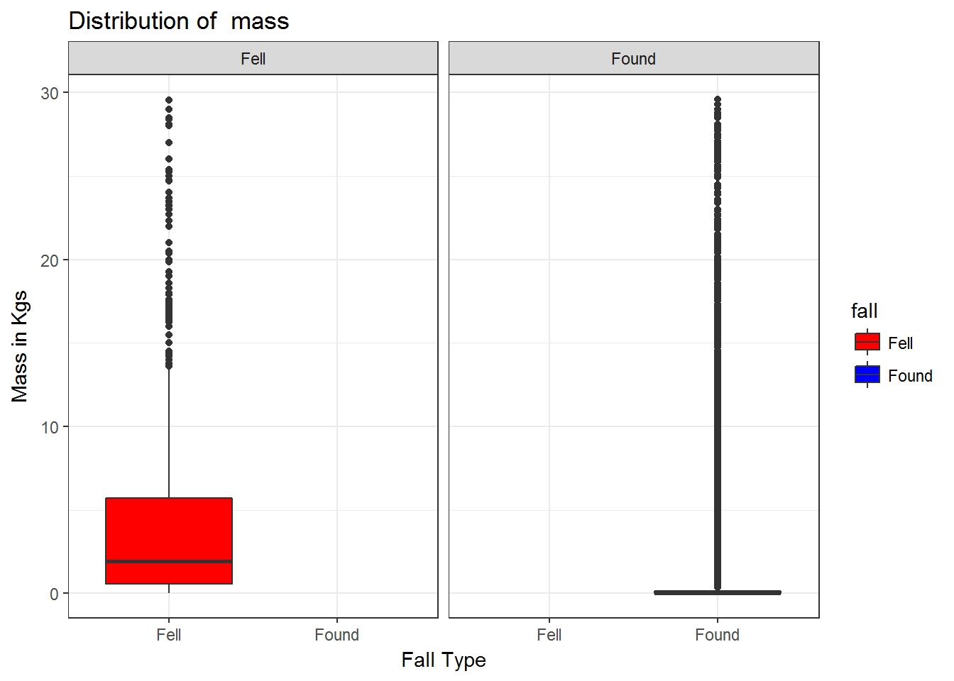
We filter the mass of the meteorites having less than 30kgs and do a boxplot.

MetLandings %>%
  mutate( fill = as.factor(fall)) %>%
  filter( (mass/1e3) < 30) %>%
      ggplot(aes(x = fall, y= mass/1e3, fill = fall)) +
      geom_boxplot() +
      scale_fill_manual( values = c("red","blue") ) +
  
      facet_wrap(~fall) +
  
      labs(x= 'Fall Type',y = 'Mass in Kgs', title = paste("Distribution of", ' mass ')) +
      theme_bw()