Chapter 8 Time of Crime

8.1 Most Crimes

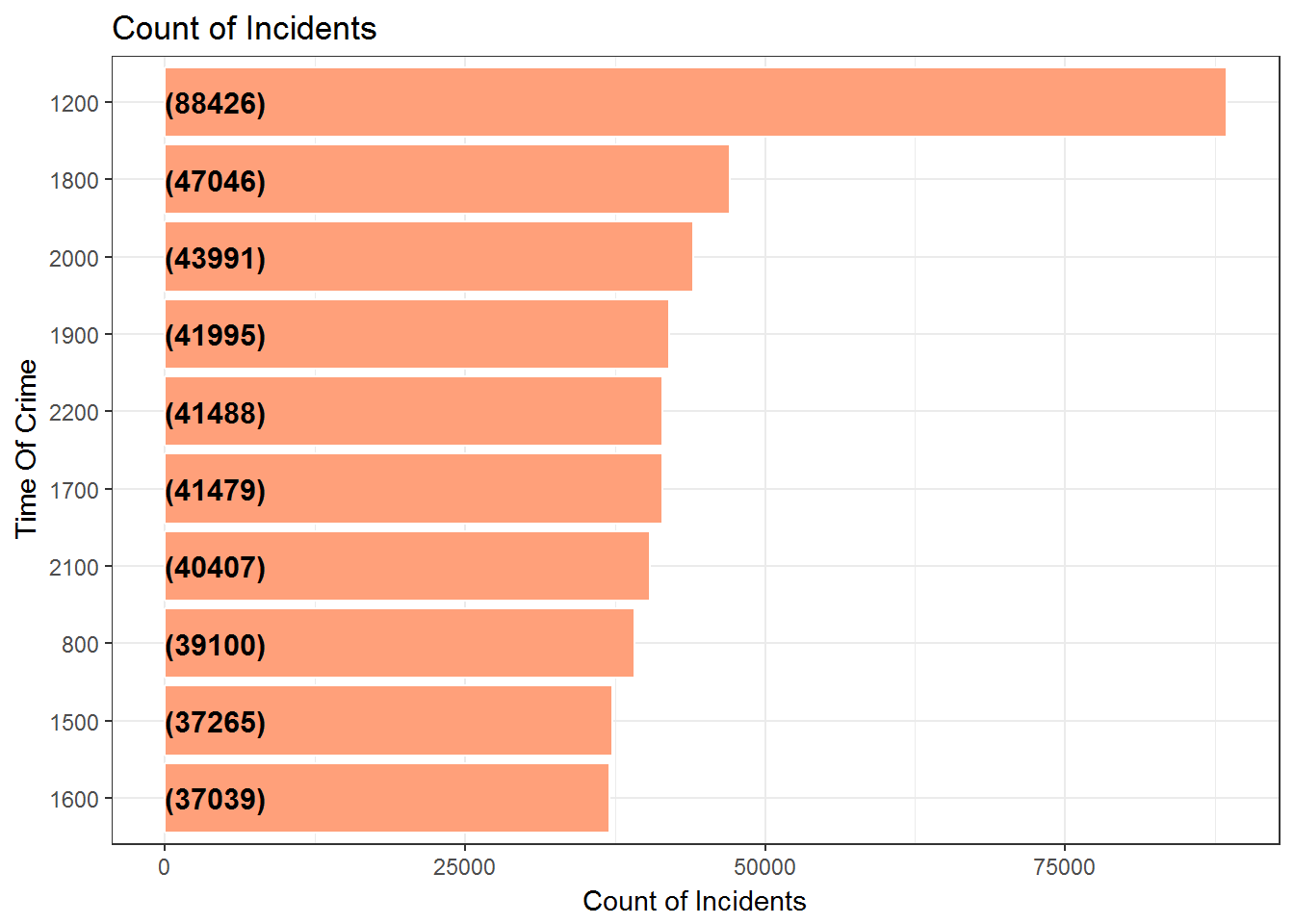
The plot shows the hours of the day where most crimes occur.

LACrime %>%
  group_by(TimeOccurred) %>%
  summarise(CountIncidents = n()) %>%
  arrange(desc(CountIncidents)) %>%
  mutate(TimeOccurred = as.integer(TimeOccurred)) %>%
  mutate(TimeOccurred = reorder(TimeOccurred,CountIncidents)) %>%
  head(10) %>%
  
  ggplot(aes(x = TimeOccurred,y = CountIncidents)) +
  geom_bar(stat='identity',colour="white", fill =fillColor) +
  geom_text(aes(x = TimeOccurred, y = 1, label = paste0("(",CountIncidents,")",sep="")),
            hjust=0, vjust=.5, size = 4, colour = 'black',
            fontface = 'bold') +
  labs(x = 'Time Of Crime', y = 'Count of Incidents', 
       title = 'Count of Incidents') +
  coord_flip() + 
  theme_bw()

Crimes occur mostly at 1200 hrs. Very Strange!, why would someone commit crime so much at the middle of the day, rather than at night.

8.2 Least Crimes

LACrime %>%
  group_by(TimeOccurred) %>%
  summarise(CountIncidents = n()) %>%
  arrange(desc(CountIncidents)) %>%
  mutate(TimeOccurred = as.integer(TimeOccurred)) %>%
  mutate(TimeOccurred = reorder(TimeOccurred,CountIncidents)) %>%
  tail(10) %>%
  
  ggplot(aes(x = TimeOccurred,y = CountIncidents)) +
  geom_bar(stat='identity',colour="white", fill =fillColor) +
  geom_text(aes(x = TimeOccurred, y = 1, label = paste0("(",CountIncidents,")",sep="")),
            hjust=0, vjust=.5, size = 4, colour = 'black',
            fontface = 'bold') +
  labs(x = 'Time Of Crime', y = 'Count of Incidents', 
       title = 'Count of Incidents') +
  coord_flip() + 
  theme_bw()

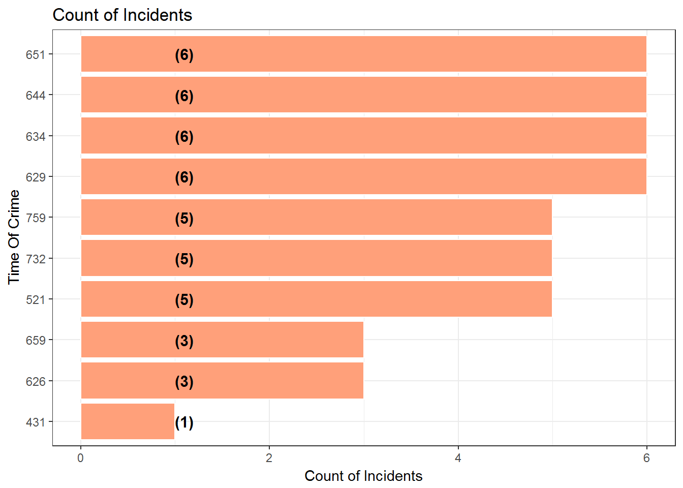
Crimes occur least at round 700 hrs. Is it because, people have woken up and getting ready for crime ? This is really interesting.

8.3 Crime Types at 1200 hrs

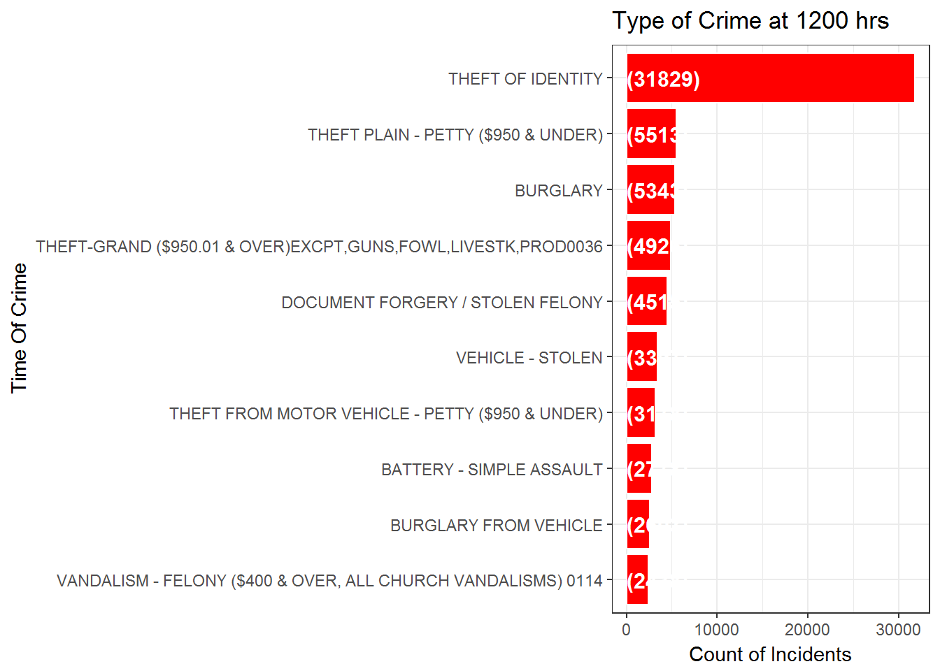
We examine the different crime types that occur at 1200 hrs since this is the time most crimes occur.

LACrime %>%
  filter(TimeOccurred == 1200) %>%
  group_by(CrimeCodeDescription) %>%
  summarise(CountIncidents = n()) %>%
  arrange(desc(CountIncidents)) %>%
  mutate(CrimeCodeDescription = reorder(CrimeCodeDescription,CountIncidents)) %>%
  head(10) %>%
  
  ggplot(aes(x = CrimeCodeDescription,y = CountIncidents)) +
  geom_bar(stat='identity',colour="white", fill = c("red")) +
  geom_text(aes(x = CrimeCodeDescription, y = 1, label = paste0("(",CountIncidents,")",sep="")),
            hjust=0, vjust=.5, size = 4, colour = 'white',
            fontface = 'bold') +
  labs(x = 'Time Of Crime', y = 'Count of Incidents', 
       title = 'Type of Crime at 1200 hrs') +
  coord_flip() + 
  theme_bw()

Theft of Identity is the most common crime type which happens during this time.